

Choose a DSCR definition before building the sheet
Use this as an illustrative term-loan basis only: DSCR = (profit after tax + depreciation + included interest) / (included principal due + included interest). Confirm the lender's numerator, denominator and period convention.
To calculate DSCR in Excel on a common Indian term-loan basis, divide profit after tax plus depreciation plus included term-loan interest by the corresponding principal due plus interest. Confirm the lender's definition. This page provides a cell layout and formulas to build your own worksheet; it does not attach a standalone Excel download.
Debt Service Coverage Ratio, or DSCR, compares the earnings or cash available for debt servicing with the debt service due in the same period. For an Indian business term-loan proposal, a commonly used profit-based calculation is: DSCR = (profit after tax + depreciation + term-loan interest) / (term-loan principal due + term-loan interest). Confirm the lender's definition before preparing the final schedule.
Do not mix this formula with a separate EBITDA or cash-flow-based approach. Different definitions can produce different results. Your sheet should state exactly which interest, non-cash adjustments and debt obligations it includes. A transparent formula is more valuable than a ratio that looks comfortable but cannot be reconciled to the projected statements.
Set up three connected worksheets
Use an Assumptions sheet, a Repayment sheet and an Annual DSCR sheet. Keep input cells distinguishable from formulas and use one amount unit throughout. Enter rupee values consistently rather than mixing actual rupees with figures in lakhs. Label the financial years and the projection start date clearly.
The assumptions should include the loan amount, annual interest rate, repayment frequency, number of instalments, disbursement date and any moratorium. Obtain these from the proposed terms or clearly label them as estimates. The simple formulas below assume one fully disbursed loan, a constant rate and monthly instalments paid at the end of each month, with no moratorium.
Calculate the monthly instalment
On Assumptions, put loan amount in B2, annual interest rate in B3 and tenure in months in B4. Enter the rate as a percentage, such as 10%, rather than the number 10. In B5 enter =PMT(B3/12,B4,-B2). The negative present value makes the returned instalment positive for this layout.
For example, B2 could contain Rs 10,00,000, B3 could contain 10% and B4 could contain 60. These are illustrative loan terms, not a lender offer. Keep the calculated instalment at full precision in the working and apply consistent rounding for display. Check how the actual lender rounds payments and adjusts the last instalment.
Build the monthly repayment schedule
On Repayment, use columns A to G for period, payment date, opening balance, instalment, interest, principal and closing balance. For the first instalment in row 2, enter period 1 in A2 and the first actual due date in B2. Use the formulas below with a positive loan balance and positive payments.
| Cell | Formula | Meaning |
|---|---|---|
| C2 | =Assumptions!B2 | Opening loan balance |
| D2 | =Assumptions!$B$5 | Monthly instalment |
| E2 | =C2*Assumptions!$B$3/12 | Monthly interest |
| F2 | =D2-E2 | Principal repaid |
| G2 | =C2-F2 | Closing balance |
In the next row, set A3 to =A2+1, B3 to =EDATE(B2,1) and C3 to =G2. Copy the instalment, interest, principal and closing formulas down for the agreed number of periods. Check the final balance and adjust the final payment if the actual rounding policy requires it. Do not extend regular instalments beyond the loan's maturity.
This monthly-rate approach is unsuitable without adjustment for daily interest, irregular dates, floating rates, staged disbursement or capitalised interest. Model those terms explicitly or use the lender's repayment schedule. Multiplying the opening loan amount by the annual rate for every year overstates interest on a reducing-balance loan.
Summarise repayments by financial year
Use the actual due dates to allocate principal and interest into April-to-March years. Do not multiply one monthly instalment by twelve if the first or final year has fewer payments. For an illustrative year from 1 April 2026 to 31 March 2027, principal can be summed using =SUMIFS(Repayment!F:F,Repayment!B:B,">="&DATE(2026,4,1),Repayment!B:B,"<"&DATE(2027,4,1)).
Use the same date criteria with Repayment!E:E for interest. The exclusive next-year start avoids ambiguity at the year boundary. Link the resulting annual interest to the projected profit and loss account, and link annual principal to the cash flow and loan balance movement. This keeps the DSCR denominator consistent with the rest of the proposal.
Create the annual DSCR block
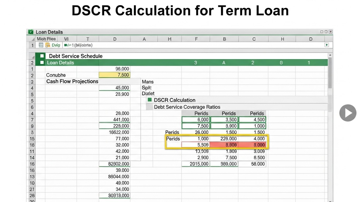
Copy this DSCR worksheet layout into Excel
Use column A for the labels below and column B for one financial year. Keep every amount in the same unit and period. Link the first four input rows to the projected statements and annual repayment summary when those schedules are available.
- A2: Profit after tax. B2: enter or link the amount.
- A3: Depreciation. B3: enter or link the amount.
- A4: Included term-loan interest. B4: link the same interest scope used for debt service.
- A5: Included principal due. B5: link the annual repayment total.
- A6: Earnings available. B6: =SUM(B2:B4)
- A7: Debt service. B7: =SUM(B4:B5)
- A8: DSCR. B8: =IF(B7=0,"N/A",B6/B7)
Test the sheet with illustrative amounts: profit after tax Rs 3,00,000, depreciation Rs 80,000, interest Rs 70,000 and principal Rs 2,30,000. Earnings available are Rs 4,50,000 and debt service is Rs 3,00,000, giving DSCR of 1.50. This is a formula check, not a prescribed bank threshold.
Copy the year column across only after checking the links. Keep zero-debt-service years visible as not applicable, and label any average according to the lender's convention. Do not add interest and depreciation again if you start from a figure that already excludes those charges.
On Annual DSCR, use each column for a financial year. Put profit after tax in row 2, depreciation in row 3, term-loan interest in row 4 and principal due in row 5. In B6 enter =SUM(B2:B4) for the numerator. In B7 enter =SUM(B4:B5) for debt service. In B8 enter =IF(B7=0,"N/A",B6/B7).
Profit after tax should already include the interest and depreciation charges before those permitted adjustments are added back. If your starting figure is EBITDA, adding the same items again would distort the numerator. Treat other non-cash items and existing loans according to the lender's agreed definition rather than inserting them automatically.
A worked annual example
Assume profit after tax is Rs 3,00,000, depreciation is Rs 80,000 and included term-loan interest is Rs 70,000. The numerator is Rs 4,50,000. If principal due is Rs 2,30,000, total debt service is Rs 3,00,000 and DSCR is 1.50. These figures are a separate annual illustration, not outputs claimed for the earlier PMT example.
If profit after tax falls to Rs 1,80,000 while the other figures remain unchanged, the numerator becomes Rs 3,30,000 and DSCR becomes 1.10. Use the change to examine repayment resilience. A lender's required minimum depends on its policy and the proposal; there is no universal sanction threshold established by this example.
Review averages and periods without repayments
An aggregate coverage measure divides total included numerators by total included debt service. It is not generally equal to the arithmetic average of annual ratios. Label the measure and follow the bank's requested convention. Show the lowest annual DSCR as well, because a comfortable aggregate can hide a weak repayment year.
Where no debt service is due, show the annual ratio as not applicable rather than zero or infinity. Review whether and how that year's numerator belongs in the requested average. A moratorium year still needs a cash-flow review, particularly where interest remains payable or later capitalisation changes the loan balance.
For the related preparation guidance, see estimate a loan amount using DSCR.
For the related preparation guidance, see EMI repayment calculator.
Check the sheet before using it in a proposal
- Total scheduled principal should reconcile to the loan amount, allowing for explicitly modelled adjustments.
- Opening balance less principal should equal closing balance each month.
- Annual principal and interest should reconcile to the monthly schedule.
- Projected interest should agree with the profit and loss account.
- All included loans should follow the same DSCR scope and period convention.
- Test lower sales, delayed collections and a higher interest rate where relevant.
DSCR is not a complete cash-flow test. Receivable delays, stock funding, capital expenditure and promoter withdrawals can create cash pressure even when the ratio exceeds one. Review the projected cash balance and working capital requirement alongside coverage.
Finxora's project report software prepares projected statements, repayment schedules and DSCR, with Excel output available for review. Compare the report samples with the bank's format. Whether you use a spreadsheet or a generated report, consistent definitions and reconciled repayment timing remain essential.